The 12 variables that we need to estimate are, $$ \mathbf{x} = \begin{bmatrix} x \\ y \\ z\\ \dot x \\ \dot y \\ \dot z \\ \phi \\ \theta \\ \psi \\ \dot \phi \\ \dot \theta \\ \dot \psi \end{bmatrix} \tag{1} $$
There are cases when you don’t need to estimate all of them and can get away with only estimating a few of them, such as when controlling the drone via radio control (RC), but I’ll leave that discussion for the “full architecture example” post. For now, let’s assume that we want to measure all of the state variables.
I’ll give 3 examples of varying complexity for measuring the state variables depending on the onboard sensors and available compute power. The first example assumes that you have a gyroscope, accelerometer, magnetometer, barometer or altimeter, and a GPS but have heavy computational constraints. The second example uses the same set of sensors but assumes that you have enough onboard processing power to perform more powerful filtering techniques such as an Extended Kalman Filter (EKF) or an Unscented Kalman Filter (UKF). The last example assumes that you are in a GPS denied environment, have onboard Lidar or stereo camera pairs, and enough compute power and implementation skills to perform ICP or visual odometry in real time.
Simple
The simplest state estimation pipeline I’ll introduce requires having a GPS with steady signal, an altimeter or barometer, and an IMU with a gyroscope, accelerometer, and magnetometer.
In order to estimate \(\phi\), \(\theta\), \(\dot \phi\), \(\dot \theta\) we will be fusing the measurements of the gyroscope and accelerometer using a complementary filter. However, it's important to realize that when we read from the gyroscope we are getting \(p\) and \(q\), not \(\dot \phi\) and \(\dot \theta\). If this notation is unfamiliar to you, see the post where we created a model of a quadcopter. We can convert the gyroscope readings at time \(p_t\), \(q_t\), and \(r_t\) to \(\dot \phi^g_t\), \(\dot \theta^g_t\), and \(\dot \psi^g_t\) as follows, $$ \begin{bmatrix} \dot \phi^g_t \\ \dot \theta^g_t \\ \dot \psi^g_t \end{bmatrix} = \begin{bmatrix}1 & S_\phi T_\theta & C_\phi T_\theta \\ 0 & C_\phi & -S_\phi \\ 0 & \frac{S_\phi}{C_\theta} & \frac{C_\phi}{C_\theta} \end{bmatrix} \begin{bmatrix} p_t \\ q_t \\ r_t \end{bmatrix} $$ where \(C_x\) denotes \(\cos(x)\), \(S_x\) denotes \(\sin(x)\), and \(T_x\) denotes \(\tan(x)\).
We'll also need to convert the accelerometer readings \(A_x\), \(A_y\), and \(A_z\) to get \(\phi^a_t\) and \(\theta^a_t\) as follows, $$ \begin{bmatrix} \phi^a_t \\ \theta^a_t \end{bmatrix} = \begin{bmatrix} \tan^{-1}(\frac{A_y}{\sqrt{A^2_x + A^2_z}}) \cdot \frac{180}{\pi} \\ \tan^{-1}(\frac{A_x}{\sqrt{A^2_y + A^2_z}}) \cdot \frac{180}{\pi} \end{bmatrix} $$ the multiplication by \(\frac{180}{\pi}\) is needed to convert from radians to degrees.
Finally, \(\phi_t\) and \(\theta_t\) can be estimated as follows using a complementary filter: $$ \begin{bmatrix} \phi_t \\ \theta_t \end{bmatrix} = \begin{bmatrix} (1 - \alpha)(\phi_{t-1} + \dot \phi^g_t \varDelta t) + \alpha \phi^a_t \\ (1 - \alpha)(\theta_{t-1} + \dot \theta^g_t \varDelta t) + \alpha \theta^a_t \end{bmatrix} $$ where \(\alpha\) is a parameter that can be tuned but will typically be around \(0.95\). See the next paragraph for a guide on tuning the alpha parameter.
The complementary filter looks like a naive weighting between the gyroscope and accelerometer but it is performing a low pass filter on the gyroscope measurement and a high pass filter on the accelerometer measurement. A great visualization along with a derivation of these equations can be seen here and a visualization of differing values for the complementary filter that may be useful for tuning can be found here.
If you are operating under the “near hover” condition as mentioned in the model post, you can make the following assumption: $$ \begin{bmatrix}1 & S_\phi T_\theta & C_\phi T_\theta \\ 0 & C_\phi & -S_\phi \\ 0 & \frac{S_\phi}{C_\theta} & \frac{C_\phi}{C_\theta} \end{bmatrix} \approx \begin{bmatrix} 1 & 0 & 0 \\ 0 & 1 & 0 \\ 0 & 0 & 1 \end{bmatrix} $$ which allows you to make the approximation that, $$ \begin{bmatrix} \dot \phi \\ \dot \theta \end{bmatrix} \approx \begin{bmatrix} p \\ q \end{bmatrix} $$ Remember that these simplifications are only valid if the drone is near hover.
The \(\psi\) value can be found using the magnetometer. As shown in the datasheet,
the main equation is
$$
\tan^{-1}({\frac{H_x}{H_y}})
$$
where \(H_y\) and \(H_x\) are the readings given from the magnetometer. Note that you will have to subtract an offset (not shown) depending on the value of \(H_y\). See the datasheet for details.
In order to find \(\dot \psi\) you can take subsequent values of \(\psi\),
$$
\dot \psi_t = \frac{\psi_t - \psi_{t - 1}}{\varDelta t}
$$
where \(\varDelta t\) is the sample rate of your magnetometer.
Magnetometers can be quite noisy so trying to accurately obtain yaw with a magnetometer may work well in an open field but may fail unexpectedly when close to metallic structures. Keep this in mind during your design and when flying.
\(x\) and \(y\) can be found via your gps. Depending on your application you may need to transform the output of your GPS to a local coordinate frame. The datasheet of your sensor should give you plenty of information on this. \(\dot x\) and \(\dot y\) can be found with differential measurements of \(x\) and \(y\) as follows, $$ \dot x = \frac{x_t - x_{t-1}}{\varDelta t} $$ $$ \dot y = \frac{y_t - y_{t-1}}{\varDelta t} $$
Z can be found with an altimeter or a barometer. If you have a barometer and are getting raw pressure measurements you should be able to look into the datasheet of your sensor to find a conversion between the output and the change in height. There are also many off the shelf altimeters sold on places like sparkfun, adafruit, and others which do this pressure conversion for you and will save you a couple of minutes of looking into the data sheet. \(\dot z\) can be found by taking differential measurements of \(z\) as follows: \(\dot z = \frac{z_t - z_{t-1}}{\varDelta t}\) where \(\varDelta t\) is the sample rate of your sensor.
Complex
The biggest difference of this approach when compared to the last one is that this one assumes that you have a model of your system. We’ll be using the model from a previous post. Covering each of the filters in this section in depth would require an entire book in itself [1], so I have opted to give an overview of each and link to more thorough references so that motivated readers can dig deeper if desired. Most of the references come from [1] which is a must read if this is your first time looking at filters for state estimation.
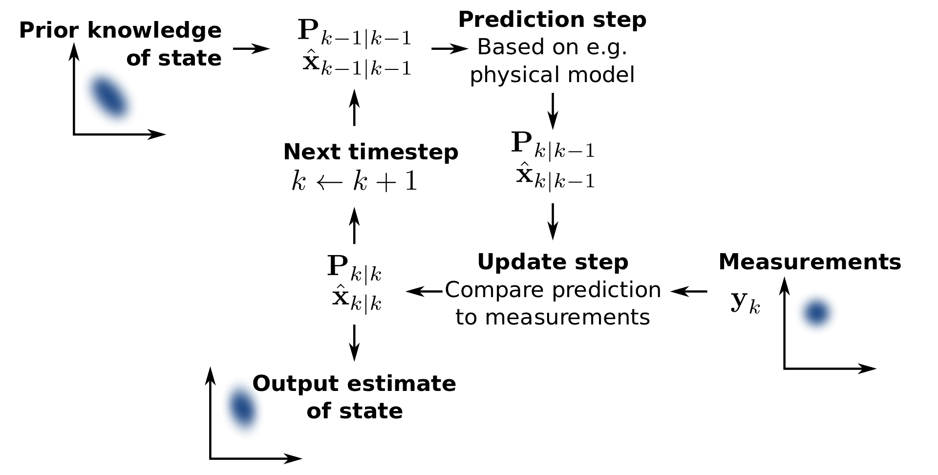
Filtering approaches usually adhere to the “Prediction-Correction” (or “Prediction-Update”) framework made famous by the Kalman Filter [4]. The main idea here is that at every time step you use your model of the system to make a prediction of the state of the system, then use the onboard sensors to measure the state of the system, and finally you combine these two states in order to obtain a more accurate state of the system. A fun fact is that the complementary filter that I introduced in the last section also adheres to this framework, though the simplified equations make it less clear. If you’re interested in investigating that, see here for details.
The Kalman Filter [3][4] is a technique that can be used to estimate the state of a linear dynamical system. Some great resources for learning about kalman filters if you haven’t studied them before are [1] and [2]. The equations of the Kalman filter are given as follows [1], $$ \begin{align} \bar{\mathbf{x}} & = \mathbf{Fx} + \mathbf{Bu}\\ \bar{\mathbf{P}} & = \mathbf{FPF^T} + \mathbf{Q}\\ \mathbf{y} & = \mathbf{z} - \mathbf{H \bar{x}}\\ \mathbf{K} & = \mathbf{\bar{P} H^T} ( \mathbf{H \bar{P} H^T} + \mathbf{R} ) ^{-1}\\ \mathbf{x} & = \mathbf{\bar{x}} + \mathbf{Ky} \\ \mathbf{P} & = (\mathbf{I} - \mathbf{KH}) \mathbf{\bar{P}} \end{align} $$
where \(\mathbf{x}\) is our system’s state. In our case it is defined by \((1)\). \(\mathbf{P}\) is the system’s covariance matrix. \(\mathbf{F}\) is our state transition function which propagates a state from time \(t\) to time \(t + 1\). \(\mathbf{K}\) is the Kalman gain which varies the weighting between our prediction and our sensor state. \(\mathbf{z}\) is the measurement from our sensors. \(\mathbf{H}\) converts the measurements of our state to what the sensor would measure. \(\mathbf{Q}\) is the process noise and \(\mathbf{R}\) is the observation noise. See chapter 6 of [1] if you are unfamiliar with these terms.
The notation here is pretty dense, but remember what the Kalman Filter is doing: it predicts where our system is supposed to be using our model then combines that with the measurement we got from our sensors to get a better estimate of our system’s state.
So now we can go ahead and put our system into this form right? Well, not quite. One important thing that I’ve glossed over is that the Kalman Filter equations above won’t work in our case since our system is nonlinear. If you aren’t sure what I mean by this, try to put our model \(\mathbf{\dot x}\) into the standard state space form, $$ \mathbf{\dot x} = \mathbf{Ax} + \mathbf{Bu} $$
Without approximating the cosine and sine terms, you won’t be able to. We could try to approximate the non-linearities created by \(\phi\) and \(\theta\) by doing a small angle approximation, but this would not be a valid approximation for \(\psi\). A small angle approximation for \(\psi\) would mean that the quadcopter yaw would always have to be in the range \(-15^{\circ} < \psi < 15^\circ\) so that the estimate does not accumulate significant error. This is too restrictive for any real world scenario.
However, there are two popular extensions to the Kalman Filter, the extended kalman filter and the unscented kalman filter, which have been created in order to extend the original Kalman Filter to problems with non-linear dynamics. Let’s look at those now.
Extended Kalman Filter
The Extended Kalman Filter (EKF) is a popular approach that came about in the 60s after Dr. Kalman proposed the Kalman Filter for linear systems. The main idea is to linearize the dynamics of your system, use some numerical integration technique to predict the state of the system after one time step, and use similar equations to those proposed by the Kalman Filter to propagate your state prediction and fuse your sensor predictions at each time step. Borrowing notation from [1], $$ \begin{align} \mathbf{F} & = \frac{\partial f(\mathbf{x}_t, \mathbf{u}_t)}{\partial \mathbf{x}}\\ \bar{\mathbf{x}} & = f(\mathbf{x}_t, \mathbf{u}_t)\\ \bar{\mathbf{P}} & = \mathbf{FPF^T} + \mathbf{Q}\\ \mathbf{H} & = \frac{\partial h(\mathbf{x}_t)}{\partial \mathbf{x}}\\ \mathbf{y} & = \mathbf{z} - h(\bar{x})\\ \mathbf{K} & = \mathbf{\bar{P} H^T} ( \mathbf{H \bar{P} H^T} + \mathbf{R} ) ^{-1}\\ \mathbf{x} & = \mathbf{\bar{x}} + \mathbf{Ky}\\ \mathbf{P} & = (\mathbf{I} - \mathbf{KH}) \mathbf{\bar{P}} \end{align} \tag 2 $$
As stated earlier, the main differences come from linearizing the dynamics to get the state transition function \(\mathbf{F}\) as well as linearizing the measurement function to get the matrix \(\mathbf{H}\). I've kept this section on the EKF purposefully sparse because I recommend using the UKF whenever possible. See chapter 11 of [1] for more details on the EKF.
Unscented Kalman Filter
The Unscented Kalman Filter (UKF) came about due to problems with the Extended Kalman Filter such as how difficult it was to tune and the computational overhead of generating the jacobians [5]. The main idea of the UKF is to choose a set of points to propagate through your nonlinear transition function such that these points give you a good enough estimate of the underlying dynamics. This sounds simple, but how do you know which points to choose? The original paper [5] proposes a method colloquially called the “Julier sigma points” for finding these points. Lastly, the unscented transform is used to propagate the state of the system even though it is a nonlinear function.
Again borrowing notation from [1], the UKF equations are, $$ \begin{align} \mathbf{\mathcal Y} & = f(\mathcal X) \\ \mathbf{\bar x} & = \sum w^m \mathbf{\mathcal Y} \\ \bar{\mathbf{P}} & = \sum w^c(\mathbf{\mathcal Y} - \mathbf{\bar x}) (\mathbf{\mathcal Y} - \mathbf{\bar x})^T + \mathbf{Q}\\ \mathbf{\mathcal Z} & = h(\mathbf{\mathcal Y}) \\ \mathbf{\mu}_z & = \sum w^m \mathbf{\mathcal Z}\\ \mathbf{y} & = \mathbf{z} - \mathbf{\mu}_z\\ \mathbf{P}_z & = \sum w^c(\mathbf{\mathcal Z} - \mathbf{\mu}_z)(\mathbf{\mathcal Z} - \mathbf{\mu}_z)^T + \mathbf{R}\\ \mathbf{K} & = [\sum w^c (\mathbf{\mathcal Y} - \mathbf{\bar x})(\mathbf{\mathcal Z} - \mathbf{\mu}_z)^T] \mathbf{P}_z^{-1}\\ \mathbf{x} & = \mathbf{\bar{x}} + \mathbf{Ky}\\ \mathbf{P} & = (\mathbf{I} - \mathbf{KH}) \mathbf{\bar{P}} \end{align} \tag 3 $$
The UKF equations look different from the EKF and the linear KF equations but they still follow the same "Prediction-Correction" framework. The biggest difference comes from the incorporation of the sigma points into both the prediction and correction steps. See chapter 10 of [1] for more details on the UKF.
I recommend using the UKF when possible since it is typically more robust to noise and easier to tune while also not having the computational overhead of calculating jacobians. Again, for those who want a more thorough introduction to using filters for state estimation see [1]. It is the best introduction and reference I have found on the topic.
More Complex
This last example assumes that your onboard sensors are either cameras or Lidar. A word of warning: the algorithms in this section are much more complicated than those in previous sections.
Lidar sensors give phenomenal range and accuracy but they come with a large price tag and design constraints that require the drone to be significantly larger. On the other hand, small consumer drones with autonomous capabilities use data from stereo cameras to implement Visual Odometry (VO) algorithms and perform state estimation.
Iterative Closest Point
The standard algorithm for state estimation using Lidar is Iterative Closest Point (ICP) which at every time step \(k\) takes as input a source lidar scan \(p\) and a target lidar scan \(q\), each with an \(n\) number of points, and tries to find the transformation \(\mathbf{T}_k\) that when applied to \(p\) best aligns it with \(q\) as measured by a least squares error. The association between a point \(p_i\) and \(q_i\) is done using a nearest neighbor approach. As an optimization problem this can be written as follows,
$$
\begin{align}
\mathbf{T}_k & = \arg \min_{\mathbf{T}_k} \sum_{i=1}^n \lVert T_k p_i - q_i \rVert_2 \\
& = \arg \min_{\mathbf{R}_k, \mathbf{t}_k} \sum_{i=1}^n \lVert \mathbf{R}_k p_i + \mathbf{t}_k - q_i \rVert_2
\end{align}
$$
where \(\mathbf{R}_k\) and \(\mathbf{t}_k\) are the rotational and translational aspects of the transformation \(\mathbf{T}_k\) defined as follows using the Z-Y-X rotation convention,
$$
\begin{align}
\mathbf{R}_k & =
\begin{bmatrix}
\cos(\gamma) \cos(\beta) & -\sin(\gamma) \cos(\alpha) + \cos(\gamma) \sin(\beta) \sin(\alpha) & \sin(\gamma) \sin(\alpha) + \cos(\gamma) \sin(\beta) \cos(\alpha)\\
\sin(\gamma) \cos(\beta) & \cos(\gamma) \cos(\alpha) + \sin(\gamma) \sin(\beta) \sin(\alpha) & -\cos(\gamma) \sin(\alpha) + \sin(\gamma) \sin(\beta) \cos(\alpha)\\
-\sin(\beta) & \cos(\beta) \sin(\alpha) & \cos(\beta) \cos(\alpha)
\end{bmatrix} \\
\mathbf{t}_k & =
\begin{bmatrix}
t_x \\ t_y \\ t_z
\end{bmatrix}
\end{align}
$$
where \(\alpha\) denotes rotation about the x-axis, \(\beta\) denotes rotation about the y-axis, and \(\gamma\) denotes rotation about the z-axis.
In order to eliminate the non-linearites of \(\mathbf{R}_k\), a small angle approximation is done which simplifies it to,
$$
\mathbf{R}_k \approx
\begin{bmatrix}
1 & -\gamma & \beta\\
\gamma & 1 & -\alpha\\
-\beta & \alpha & 1\\
\end{bmatrix}
$$
There are two popular variants of ICP: point-to-point and point-to-plane.
Point-to-point ICP
Intuitively, point-to-point ICP tries to align every point \(p_i\) with its corresponding point in \(q_i\). As mentioned previously, these point correspondences are found using a nearest-neighbor approach.
From section 2.6.2 of [11] the point-to-point ICP problem is solved by first finding the centroids of the point clouds,
$$
\begin{align}
\mu_p & = \frac{1}{n} \sum_{i=1}^n p_i \\
\mu_q & = \frac{1}{n} \sum_{i=1}^n q_i
\end{align}
$$
using this to create the covariance matrix \(\mathbf{H}\),
$$
\mathbf{H} = \sum_{i=1}^n (p_i - \mu_p)(q_i - \mu_q)^T
$$
then performing a Singular Value Decomposition on \(\mathbf{H}\) such that,
$$
\mathbf{H} = \mathbf{U} \Lambda \mathbf{V}^T
$$
With this in hand, \(\mathbf{R}_k\) and \(\mathbf{t}_k\) are found as follows,
$$
\begin{align}
\mathbf{R}_k & = \mathbf{V} \mathbf{U}^T \\
\mathbf{t}_k & = \mu_q - \mathbf{R}_k \mu_p
\end{align}
$$
See here for a visualization of point to point ICP and see [11] for more details.
Point-to-plane ICP
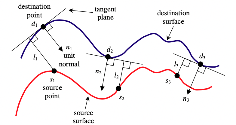
Point to plane ICP also finds corresponding points by nearest neighbor but it instead tries to minimize the distance between every point \(p_i\) and the plane defined by its corresponding point \(q_i\). In this case the optimization problem becomes,
$$
\begin{align}
\mathbf{T}_k & = \arg \min_{\mathbf{T}_k} \sum_{i=1}^n \lVert (T_k p_i - q_i ) \cdot \mathbf{n}_i\rVert_2 \\
& = \arg \min_{\mathbf{R}_k, \mathbf{t}_k} \sum_{i=1}^n \lVert (\mathbf{R}_k p_i + \mathbf{t}_k - q_i) \cdot \mathbf{n}_i \rVert_2
\end{align}
$$
where \(\mathbf{n}_i\) is the normal vector of the surface at point \(q_i\).
The intuition behind this slight variation to the problem is that the point to plane metric assumes that the corresponding points come from the same surface whereas the point to point metric makes the unlikely assumption that they are in fact the same point. From section 2.6.2 of [11], point-to-plane ICP is solved by first creating the matrix \(\mathbf{G}\) and vector \(\mathbf{h}\) such that,
$$
\begin{align}
\mathbf{G} & =
\begin{bmatrix}
\cdots p_i \times \mathbf{n}_i \cdots \\
\cdots \mathbf{n}_i \cdots
\end{bmatrix} \\
\\
\mathbf{h} & =
\begin{bmatrix}
\vdots \\
(q_i - p_i) \cdot \mathbf{n}_i\\
\vdots
\end{bmatrix}
\end{align}
$$
and solving,
$$
\mathbf{G} \mathbf{G}^T \mathbf{\tau} = \mathbf{G} \mathbf{h}
$$
for \(\tau\) which gives,
$$
\mathbf{\tau} =
\begin{bmatrix}
\alpha \\ \beta \\ \gamma \\ t_x \\ t_y \\ t_z
\end{bmatrix} =
(\mathbf{G} \mathbf{G}^T)^{-1} \mathbf{G} \mathbf{h}
$$
Now that we have \(\tau\), we can use the definitions of \(\mathbf{R}_k\) and \(\mathbf{t}_k\) to get our answer.
See [10] for a succint overview of point-to-plane ICP and see [11] for an exhaustive resource of point cloud data association algorithms.
Visual Odometry
Visual Odometry (VO) is an alternative to Lidar when a camera is present. VO itself requires a whole post to explain so I’ll give a high level overview of one example pipeline here along with a handful of references for those who are eager to dive into it. If there's enough interest, I’ll go in depth in a later post.
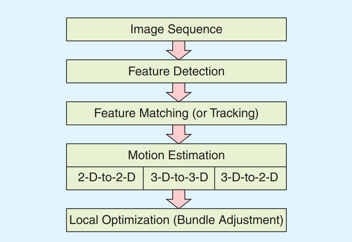
As shown in [6] and [7], at each time step \(k\) the typical VO pipeline goes as follows:
1) Capture new image \(I_k\)
2) Extract and match features between \(I_{k-1}\) and \(I_k\)
3) Compute essential matrix \(\mathbf{E}\) for \(I_{k-1}\) and \(I_k\)
4) Compute rotation \(\mathbf{R}_k\) and translation \(\mathbf{t}_k\) from \(\mathbf{E}\) and create transformation matrix \(\mathbf{T}_k\)
5) Relative scale computation
6) Concatenate transformation, \(\mathbf{C}_k = \mathbf{C}_{k-1} \mathbf{T}_k\)
7) Repeat from step 1
In this case a subscript \(k\) denotes the time step, a subscript \(I\) denotes an image, and \(C_k\) denotes your pose at time step \(k\).
The features that are extracted in step 2 may be SIFT, ORB, etc. If you’re unfamiliar with these, see here. See the slide titled “2D to 2D - Relative Scale Computation” in [7] for details on step 5.
Again, I may write a post describing VO in detail since there is a lot more to be said, but if you want to dig deeper right now see [6] and [7].
Some Suggestions
The time and expertise required to implement a simple state estimation technique is significantly less than some state of the art methods. However, it’s not always clear when a system will respond well with a more advanced approach. I believe that simpler is better in most engineering projects and this especially holds true for choosing a state estimation technique. Most quadcopters will get great results using the first approach shown above even though it’s quite simple. Moreover, the EKF is infamously hard to tune and many papers show that for quadcopters a complementary filter will give comparable results [9]. The goal of any project should be to get the best results in the amount of time you have, and sometimes going for the most advanced approach will cause more headaches with minimal gain. If you intend to implement the techniques shown in this post I suggest starting with the simple techniques and only going to the more advanced after tuning and not obtaining sufficient results.
For those that want a different look at these topics, a short write up can be found in [8]. In the next post we’ll start talking about motion planning by introducing a special property of quadcopters called differential flatness which will make our lives a lot easier when we start thinking about planning trajectories.
References
[1] https://github.com/rlabbe/Kalman-and-Bayesian-Filters-in-Python
[2] https://www.kalmanfilter.net/default.aspx
[3] https://en.wikipedia.org/wiki/Kalman_filter
[4] Kalman, R. E. (March 1, 1960). "A New Approach to Linear Filtering and Prediction Problems." ASME. J. Basic Eng. March 1960; 82(1): 35–45. https://www.cs.unc.edu/~welch/kalman/media/pdf/Kalman1960.pdf
[5] E. A. Wan and R. Van Der Merwe, "The unscented Kalman filter for nonlinear estimation," Proceedings of the IEEE 2000 Adaptive Systems for Signal Processing, Communications, and Control Symposium (Cat. No.00EX373), 2000, pp. 153-158, doi: 10.1109/ASSPCC.2000.882463. https://groups.seas.harvard.edu/courses/cs281/papers/unscented.pdf
[6] D. Scaramuzza and F. Fraundorfer, "Visual Odometry [Tutorial]," in IEEE Robotics & Automation Magazine, vol. 18, no. 4, pp. 80-92, Dec. 2011, doi: 10.1109/MRA.2011.943233. https://ieeexplore.ieee.org/document/6096039
[7] http://rpg.ifi.uzh.ch/visual_odometry_tutorial.html
[8] http://philsal.co.uk/projects/imu-attitude-estimation
[9] Tariqul Islam, Md. Saiful Islam, Md. Shajid-Ul-Mahmud, and Md Hossam-E-Haider , "Comparison of complementary and Kalman filter based data fusion for attitude heading reference system", AIP Conference Proceedings 1919, 020002 (2017) https://aip.scitation.org/doi/pdf/10.1063/1.5018520
[10] Low, Kok-Lim. (2004). Linear Least-Squares Optimization for Point-to-Plane ICP Surface Registration. https://www.comp.nus.edu.sg/~lowkl/publications/lowk_point-to-plane_icp_techrep.pdf
[11] François Pomerleau, Francis Colas, Roland Siegwart. A Review of Point Cloud Registration Al- gorithms for Mobile Robotics. Foundations and Trends in Robotics, Now Publishers, 2015, 4 (1), pp.1–104. 10.1561/2300000035 . hal-01178661 https://hal.archives-ouvertes.fr/hal-01178661/document