The first step to making any system autonomous is to make a model of it. Once you have a model, any number of forward integration techniques can be used to simulate it. The good news is that the simulation tends to be the easy part since there exists software such as scipy and Matlab which will integrate your model dynamics with minimal effort on your part for most systems. The bad news is that creating the model can be challenging. Luckily we have years of research into quadcopters to lean on.
Like the rest of this series of posts, I'm going to show the equations then move on to giving you an intuitive understanding of why they are correct. There is plenty of literature that provides a rigorous look at the topic so for those who want a more thorough derivation here is the paper I’m using as a reference [1] and see [2]. The rest of this post combines ideas from those papers in order to introduce the standard model of a quadcopter. I’ll try to use the same notation where possible so that referencing the papers is straightforward.
Definitions
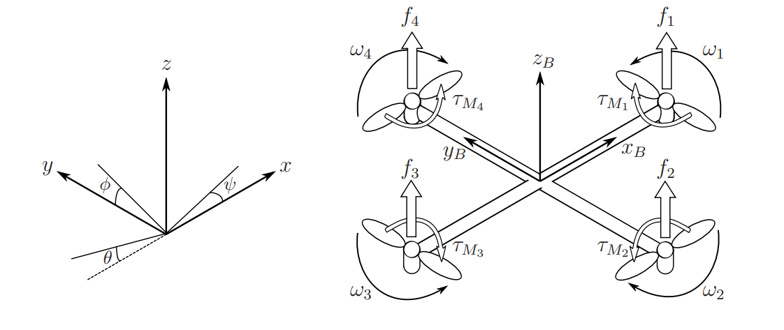
So how do simulators like Gazebo and jMavSim model a quadcopter? The first step is to figure out what we care about i.e. which variables we should keep track of. Normally we want the position and orientation of our quadcopter along with the time derivatives of each of these. Thus we can define our state \(X\) in the world frame as, $$X = \begin{bmatrix} x \\ y \\ z\\ \dot x \\ \dot y \\ \dot z \\ \phi \\ \theta \\ \psi \\ \dot \phi \\ \dot \theta \\ \dot \psi \end{bmatrix} \tag{1}$$ where \(x\), \(y\), \(z\) denote the position of the center of mass and \(\phi\), \(\theta\), and \(\psi\) denote the roll, pitch, and yaw respectively. We are able to control this state using the following control inputs, $$u = \begin{bmatrix} f_1 \\ f_2 \\ f_3 \\ f_4 \\ \end{bmatrix} $$ where \(f_i\) denotes the force provided by motor \(i\) as seen in figure 1. Motor forces are related to the motor's rpm by, $$ f_i = c_T \omega_i^2$$ where \(\omega_i\) denotes the rotations per minute (rpm) of the motor and \(c_T\) is the thrust coefficient typically determined empirically.
However, it is more common to instead command thrust and roll, pitch, and yaw torques. This leads to an alternative formulation of the control input, $$u = \begin{bmatrix} f_t \\ \tau_\phi \\ \tau_\theta \\ \tau_\psi \end{bmatrix}$$ where \(f_t\) defined as the total thrust like so, $$ f_t = \sum_{i=1}^4 f_i = \sum_{i=1}^4 c_T \omega_i^2 $$ Assuming the motor configuration shown in figure 1, this formulation is related to the motor rpms by, $$ u = \begin{bmatrix} f_t \\ \tau_\phi \\ \tau_\theta \\ \tau_\psi \\ \end{bmatrix} = \begin{bmatrix} c_T & c_T & c_T & c_T\\ 0 & -l c_T & 0 & l c_T \\ -l c_T & 0 & l c_T & 0 \\ -c_Q & c_Q & -c_Q & c_Q \end{bmatrix} \begin{bmatrix} \omega_1^2 \\ \omega_2^2 \\ \omega_3^2 \\ \omega_4^2 \\ \end{bmatrix} \tag{2} $$ as shown in [1] and [2] where \(l\) is the length of an arm and \(c_Q\) is the moment coefficient typically determined empirically. This equation can be inverted to find the required motor rpms for a desired input with the following equation, $$ u = \begin{bmatrix} \omega_1^2 \\ \omega_2^2 \\ \omega_3^2 \\ \omega_4^2 \\ \end{bmatrix} = \begin{bmatrix} \frac{1}{4 c_T} & 0 & \frac{-1}{2 l c_T} & \frac{-1}{4 c_Q}\\ \frac{1}{4 c_T} & \frac{-1}{2 l c_T} & 0 & \frac{1}{4 c_Q} \\ \frac{1}{4 c_T} & 0 & \frac{1}{2 l c_T} & \frac{-1}{4 c_Q} \\ \frac{1}{4 c_T} & \frac{1}{2 l c_T} & 0 & \frac{1}{4 c_Q} \end{bmatrix} \begin{bmatrix} f_t \\ \tau_\phi \\ \tau_\theta \\ \tau_\psi \\ \end{bmatrix} \tag{3} $$
Most planners will use thrust, roll, pitch, and yaw to plan then they will solve for the corresponding motor rpm values. Finally they will feed this into a digital to analog converter which speaks directly with the motor. Later posts on motion planning, control, and example quadcopter pipelines will go more into depth on these details.
Frames of Reference
It's important to notice that there are two frames of reference at play in our model: there is the world reference frame, which is shown on the left in figure 1, and there is the body reference frame which is attached to the quadcopter's center of mass as shown on the right side of figure 1. Our state \(X\) is in the world frame but some of the measurements we'll use to find our roll and pitch angles, such as measurements from the gyro or accelerometer, will be in the body frame. For our model we'll need to define the angular velocities in the body frame, $$ \nu = \begin{bmatrix} p \\ q \\ r \end{bmatrix} \tag{4} $$ and the angular accelerations in the body frame, $$ \dot \nu = \begin{bmatrix} \dot p \\ \dot q \\ \dot r \end{bmatrix} \tag{5} $$ where \(p\) denotes the angular velocity about the \(x\) axis, \(q\) denotes the angular velocity about the \(y\) axis, and \(r\) denotes the angular velocity about the \(z\) axis in the body frame.Now that we understand the reference frames, we'll need a rotation matrix to convert angles between the body frame and the world frame. Using the Z-Y-X rotation convention we get, $$R_B^W = \begin{bmatrix} C_\psi C_\theta & C_\psi S_\theta S_\phi - S_\psi C_\phi & C_\psi S_\theta C_\phi + S_\psi S_\phi \\ S_\psi C_\theta & S_\psi S_\theta S_\phi + C_\psi C_\phi & S_\psi S_\theta C_\phi - C_\psi S_\phi \\ -S_\theta & C_\theta S_\phi & C_\theta C_\phi \end{bmatrix} \tag{6}$$ where \(R_B^W\) denotes the rotation from the body frame to the world frame and \(C_x\) and \(S_x\) denote \(\cos(x)\) and \(\sin(x)\) respectively.
We'll also need to convert rotational velocities from the world frame to the body frame, $$ W_W^B = \begin{bmatrix}1 & 0 & -S_\theta \\ 0 & C_\phi & C_\theta S_\phi \\ 0 & -S_\phi & C_\theta C_\phi \end{bmatrix} \tag{7} $$ and from the body frame to world frame, $$ W_B^W = \begin{bmatrix}1 & S_\phi T_\theta & C_\phi T_\theta \\ 0 & C_\phi & -S_\phi \\ 0 & \frac{S_\phi}{C_\theta} & \frac{C_\phi}{C_\theta} \end{bmatrix} \tag{8} $$ As a reminder, \(C_x\) denotes \(\cos(x)\), \(S_x\) denotes \(\sin(x)\), and \(T_x\) denotes \(\tan(x)\). When \(\theta\) and \(\phi\) are near zero, also known as the "near-hover" condition, \(W_B^W\) and \(W_W^B\) are approximately equal to the identity matrix which allows us to make the assumption that $$ \begin{bmatrix} \dot \phi \\ \dot \theta \\ \dot \psi \end{bmatrix} \approx \begin{bmatrix} p \\ q \\ r \end{bmatrix} $$ Remember that this assumption is only valid when near hover.
State Space Equation
Because our state is, $$X = \begin{bmatrix} x \\ y \\ z\\ \dot x \\ \dot y \\ \dot z \\ \phi \\ \theta \\ \psi \\ \dot \phi \\ \dot \theta \\ \dot \psi \end{bmatrix} $$ the state space ODE we are looking for is, $$\dot X = \begin{bmatrix} \dot x \\ \dot y \\ \dot z \\ \ddot x \\ \ddot y \\ \ddot z \\ \dot \phi \\ \dot \theta \\ \dot \psi \\ \ddot \phi \\ \ddot \theta \\ \ddot \psi \end{bmatrix}$$ Notice that our state includes \(\dot x\), \(\dot y\), \(\dot z\), \(\dot \phi\), \(\dot \theta\), \(\dot \psi\), which means that the only values we need to solve for are \(\ddot x\), \(\ddot y\), \(\ddot z\), \(\ddot \phi\), \(\ddot \theta\), \(\ddot \psi\). As shown in [1], we can solve for these using the Newton-Euler equations to get, $$ \begin{bmatrix} \ddot x \\ \ddot y \\ \ddot z \end{bmatrix} = -g \begin{bmatrix} 0 \\ 0 \\ 1 \end{bmatrix} + \frac{f_t}{m} \begin{bmatrix} C_\psi S_\theta C_\phi + S_\psi S_\phi\\ S_\psi S_\theta C_\phi - C_\psi S_\phi \\ C_\theta C_\phi \end{bmatrix} \tag{9} $$ and, $$ \begin{bmatrix} \ddot \phi \\ \ddot \theta \\ \ddot \psi \end{bmatrix} = \begin{bmatrix} 0 & \dot \phi C_\phi T_\theta + \frac{\dot \theta S_\phi}{C_\theta^2} & -\dot \phi S_\phi C_\theta + \frac{\dot \theta C_\phi}{C_\theta^2} \\ 0 & -\dot \phi S_\phi & -\dot \phi C_\phi \\ 0 & \frac{\dot \phi C_\phi}{C_\theta} + \frac{\dot \phi S_\phi T_\theta}{C_\theta} & \frac{-\dot \phi S_\phi}{C_\theta} + \frac{\dot \theta C_\phi T_\theta}{C_\theta} \end{bmatrix} \nu + W_B^W \dot \nu \tag{10} $$ where, $$ \dot \nu = \begin{bmatrix} \dot p \\ \dot q \\ r \end{bmatrix} = \begin{bmatrix} \frac{(I_y - I_z)qr}{I_x} + \frac{\tau_\phi}{I_x} \\ \frac{(I_z - I_x)pr}{I_y} + \frac{\tau_\theta}{I_y} \\ \frac{(I_x - I_y)pq}{I_z} + \frac{\tau_\psi}{I_z} \end{bmatrix} $$ \(I_x\) is the moment of inertia about the x axis, \(I_y\) is the moment of inertia about the y axis, \(I_z\) is the moment of inertia about the z axis, \(g = 9.81\) \(m/s^2\) is the force of gravity, and \(m\) is the mass of the quadcopter. With this our state space ODE becomes, $$\dot X = \begin{bmatrix} \dot x \\ \dot y \\ \dot z \\ \dot \phi \\ \dot \theta \\ \dot \psi \\ \frac{f_t(C_\psi S_\theta C_\phi+ S_\psi S_\phi)}{m} \\ \frac{f_t(S_\psi S_\theta C_\phi - C_\psi S_\phi)}{m} \\ \frac{f_t C_\theta C_\phi}{m} - g \\ \tiny{q(\dot \phi C_\phi T_\theta + \frac{\dot \theta S_\phi}{C_\theta^2}) + r(-\dot \phi S_\phi C_\theta + \frac{\dot \theta C_\phi}{C_\theta^2}) + \frac{(I_y - I_z)}{I_x}q r + \frac{\tau_\phi}{I_x} + (\frac{(I_z - I_x)}{I_y}p r + \frac{\tau_\theta}{I_y})S_\phi T_\theta + (\frac{(I_x - I_y)}{I_z}p q + \frac{\tau_\psi}{I_z}) C_\phi T_\theta} \\ \tiny{-q \dot \phi S_\phi - \dot \phi C_\phi r + (\frac{(I_z - I_x)}{I_y}p r + \frac{\tau_\theta}{I_y}) C_\phi - (\frac{(I_z - I_x)}{I_y}p r + \frac{\tau_\theta}{I_y}) S_\phi} \\ \tiny{q(\frac{\dot \phi C_\phi}{C_\theta} + \frac{\dot \phi S_\phi T_\theta}{C_\theta}) + r(\frac{-\dot \phi S_\theta}{C_\theta} + \frac{\dot \theta C_\phi T_\theta}{C_\theta}) + \frac{(\frac{(I_z - I_x)}{I_y}p r + \frac{\tau_\theta}{I_y})S_\phi}{C_\theta} + \frac{(\frac{(I_x - I_y)}{I_z}p q + \frac{\tau_\psi}{I_z}) C_\phi}{C_\theta}} \end{bmatrix} \tag{11}$$ Yikes, those last 3 terms are nasty - good thing browsers have a zoom button. At least if you go to implement this you can type it in once then wrap it in a function call. Or you can just use the code I implement in the next post. Lastly, if you're following along with [1], you'll notice that I omitted the "gyroscopic force" since it is not normally included in the Newton-Euler equations.Intuition
I know this was a whirlwind tour and the equations popped out of nowhere so let me try to give you some intuition as to why they make sense.
The first thing I want to point out is how the equations simplify when you are near hover i.e. when \(\dot x = 0\), \(\dot y = 0\), \(\dot z = 0\), \(\phi = 0\), \(\theta = 0\), \(\psi = 0\), \(\dot \phi = 0\), \(\dot \theta = 0\), \(\dot \psi = 0\), \(f_t = mg\), \(\tau_\phi = 0\), \(\tau_\theta = 0 \), and \(\tau_\psi = 0 \). In this case, \(\dot X\) becomes the zero vector which causes \(X\) to be constant. This is what you should expect since in the ideal case when a quadcopter is hovering it just, well, hovers... It doesn't move side to side, or roll, or do anything else besides being perfectly still. Similarly, if \(f_t > mg\), then the only non-zero element of \(\dot X\) is \(\ddot z\) which means that the quadcopter will fly straight up. Finally, if we set the thrust \(f_t = 0\), the quadcopter goes into freefall.
The second case I want to point out occurs when the quadcopter is hovering but it then wants to rotate about one axis. Let's say we want the quadcopter to roll which corresponds to a rotation about the \(x\)-axis. We can force the quadcopter to do this by feeding it a non-zero \(\tau_\phi\) term. So what does \(\dot X\) give us in this case? After simplifying the equations you'll realize that the only non-zero term is \(\ddot \phi\) which is caused by the non-zero \(\tau_\phi\) term. This makes sense since that's exactly what is needed to get the quadcopter to roll. The same argument applies for rotation about the \(y\) and \(z\) axes except that they cause \(\ddot \theta\) and \(\ddot \psi\) to be non-zero due to the non-zero \(\tau_\theta\) or \(\tau_\psi\) terms.
Our intuition is correct for some common cases but if this explanation doesn't quite satisfy you, take a look at [1]. It's a great paper and I made sure to use mostly the same notation so that you can focus on the derivation and less on the notation.
In the next post I'll walk you through an implementation that I made using this model that allows for simulating a quadcopter with arbitrary motor inputs. See you there.
References
[1] Teppo Luukkonen. Modelling and control of quadcopter. Independent research project in applied mathematics, 2011. https://sal.aalto.fi/publications/pdf-files/eluu11_public.pdf
[2] Mellinger, Daniel, et al. “Trajectory Generation and Control for Precise Aggressive Maneuvers with Quadrotors.” The International Journal of Robotics Research, vol. 31, no. 5, Apr. 2012, pp. 664–674, doi:10.1177/0278364911434236.