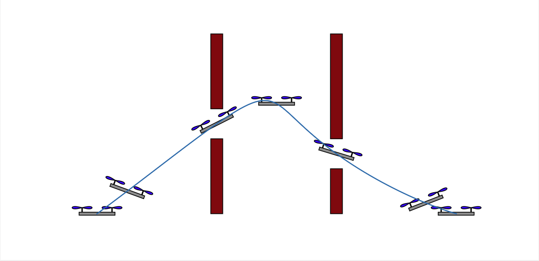
Quadcopters exhibit a property called Differential Flatness. A system that has Differential Flatness allows you to solve for some of the state variables in terms of other state variables. In the case of a quadcopter, this means that if you give me a trajectory \(x(t)\), \(y(t)\), \(z(t)\), and \(\psi(t)\) of a quadcopter, I can tell you what the other state variables of the quadcopter are at every point in the trajectory. The only caveat for quadcopters is that the trajectory must be differentiable 4 times at every given point. If you haven’t encountered differential flatness before, see section 10.8.1 of [1] for a quick overview.
As shown in section 2.3.2 of [2], let \(\sigma\) be our flat outputs which we assume are known,
$$
\sigma =
\begin{bmatrix}
\sigma_1 \\ \sigma_2 \\ \sigma_3 \\ \sigma_4
\end{bmatrix} =
\begin{bmatrix}
x \\ y \\ z \\ \psi
\end{bmatrix}
$$
Note that we also assume we know \(\dot \sigma\), \(\ddot \sigma\), \(\dddot \sigma\), and \(\ddddot \sigma\). With these assumptions, we want to solve for \(\phi\), \(\dot \phi\), \(\ddot \phi\), \(\theta\), \(\dot \theta\), and \(\ddot \theta\).
Solving for \(\phi\) and \(\theta\)
To start let,
$$
\textbf{z}_B = \frac{\textbf{t}}{\lVert \textbf{t} \rVert}
$$
where,
$$
\textbf{t} =
\begin{bmatrix}
\ddot x \\
\ddot y \\
\ddot z + g
\end{bmatrix}
$$
and \(g\) is gravity. Additionally, let
$$
\textbf{x}_C =
\begin{bmatrix}
\cos(\psi) \\ \sin(\psi) \\ 0
\end{bmatrix}
$$
and
$$
\textbf{y}_B = \frac{\textbf{z}_B \times \textbf{x}_C}{\lVert \textbf{z}_B \times \textbf{x}_C \rVert}
$$
and
$$
\textbf{x}_B = \textbf{y}_B \times \textbf{z}_B
$$
This allows us to define,
$$
R_B^W = \begin{bmatrix} \textbf{x}_B & \textbf{y}_B & \textbf{z}_B \end{bmatrix}
$$
which can be used to solve for \(\phi\) and \(\theta\) by noting that,
$$
R_B^W = \begin{bmatrix}
\cos(\psi) \cos(\theta) - \sin(\phi) \sin(\psi) \sin(\theta) & -\cos(\phi) \sin(\psi) & \cos(\psi) \sin(\theta) + \cos(\theta) \sin(\phi) \sin(\psi) \\
\cos(\theta) \sin(\psi) + \cos(\psi) \sin(\phi) \sin(\theta) & \cos(\phi) \cos(\psi) & \sin(\psi) \sin(\theta) - \cos(\psi) \cos(\theta) \sin(\phi) \\
-\cos(\phi) \sin(\theta) & \sin(\phi) & \cos(\phi) \cos(\theta)
\end{bmatrix}
$$
from the definition of Z - X - Y Euler angles. Therefore,
$$
\begin{align}
\phi & = \sin^{-1}(\textbf{y}_{B_3}) \\
\theta & = \cos^{-1}(\frac{\textbf{z}_{B_3}}{\cos(\phi)})
\end{align}
$$
where \(\textbf{y}_{B_3}\) denotes the third element of the \(\textbf{y}_B\) vector and \(\textbf{z}_{B_3}\) denotes the third element of the \(\textbf{z}_B\) vector.
Solving for \(\dot \phi\) and \(\dot \theta\)
We can also define,
$$
\textbf{h}_\omega = \frac{m}{u_1} (\dot{\textbf{a}} - (\textbf{z}_B \cdot \dot{\textbf{a}})\textbf{z}_B)
$$
where \(u_1\) is the total thrust and,
$$
\dot{\textbf{a}} = \begin{bmatrix} \dddot x \\ \dddot y \\ \dddot z \end{bmatrix}
$$
commonly referred to as Jerk.
This allows us to define,
$$
\begin{align}
p & = -\textbf{h}_\omega \cdot \textbf{y}_B \\
q & = \textbf{h}_\omega \cdot \textbf{x}_B \\
r & = \dot \psi \textbf{z}_W \cdot \textbf{z}_B
\end{align}
$$
where \(\textbf{z}_W\) is defined as the unit vector pointing in the direction of the z-axis in the world frame.
We can then use the following equation to get \(\dot \phi\) and \(\dot \theta\),
$$
\begin{bmatrix}\dot \phi \\ \dot \theta \\ \dot \psi \end{bmatrix} =
\begin{bmatrix} \textbf{x}_C & \textbf{y}_B & \textbf{z}_W \end{bmatrix}^{-1} \textbf{R}_B^W \begin{bmatrix}p \\ q \\r \end{bmatrix}
$$
Solving for \(\ddot \phi\) and \(\ddot \theta\)
To solve for \(\ddot \phi\) and \(\ddot \theta\), let
$$
\begin{align}
\omega_{BW} & = \begin{bmatrix} \textbf{x}_C & \textbf{y}_C & \textbf{z}_W \end{bmatrix} \begin{bmatrix} \dot \phi \\ \dot \theta \\ \dot \psi \end{bmatrix}\\
\omega_{CW} & = \dot \psi \textbf{z}_W
\end{align}
$$
as well as,
$$
\begin{align}
\dot u_1 & = \textbf{z}_B \cdot m \dot{\textbf{a}} \\
\ddot u_1 & = \textbf{z}_B \cdot m \ddot{\textbf{a}} - \textbf{z}_B \cdot (\omega_{BW} \times \omega_{BW} \times u_1 \textbf{z}_B) \\
\textbf{h}_{\alpha} & = \alpha_{BW} \times \textbf{z}_B = \frac{1}{u_1}(m \ddot{\textbf{a}} - \ddot u_1 \textbf{z}_B - 2 \omega_{BW} \times \dot u_1 \textbf{z}_B - \omega_{BW} \times \omega_{BW} \times u_1 \textbf{z}_B)
\end{align}
$$
where,
$$
\ddot{\textbf{a}} = \begin{bmatrix} \ddddot x \\ \ddddot y \\ \ddddot z \end{bmatrix}
$$
commonly referred to as Snap.
Now we can define,
$$
\begin{align}
\dot p & = -\textbf{h}_{\alpha} \cdot \textbf{y}_B \\
\dot q & = \textbf{h}_{\alpha} \cdot \textbf{x}_B
\end{align}
$$
Finally, we can solve for \(\dot r\) using the third equation from the following nasty system of equations,
$$
R_B^W (\begin{bmatrix} \dot p \\ \dot q \\ \dot r \end{bmatrix} + \begin{bmatrix} p \\ q \\ r \end{bmatrix} \times \begin{bmatrix} p \\ q \\ r \end{bmatrix}) =
\omega_{CW} \times \dot \phi \textbf{x}_c + \omega_{BW} \times \dot \theta \textbf{y}_B + \begin{bmatrix} \textbf{x}_C & \textbf{y}_B & \textbf{z}_W \end{bmatrix} \begin{bmatrix} \ddot \phi \\ \ddot \theta \\ \ddot \psi \end{bmatrix}
$$
Remember that we are given \(\ddot \psi\) which is what allows us to solve for \(\dot r\).
See section 2.3.2 of [2] and section \(III\) of [3] for a more in-depth derivation of the equations shown in this post.
Summary
With these equations in hand, we are now able to determine the entire state of a quadcopter knowing only \(x\), \(y\), \(z\), \(\psi\) and their derivatives with respect to time (each differentiated 4 times). The usefulness of these equations will be clear in the next post where we do motion planning. See you there.
References
[1] Russ Tedrake. Underactuated Robotics: Algorithms for Walking, Running, Swimming, Flying, and Manipulation (Course Notes for MIT 6.832). Downloaded on 6/4/22 from http://underactuated.mit.edu/
[2] Mellinger, Daniel Warren, "Trajectory Generation and Control for Quadrotors" (2012). Publicly Accessible Penn Dissertations. 547. https://repository.upenn.edu/edissertations/547
[3] D. Mellinger and V. Kumar, "Minimum snap trajectory generation and control for quadrotors," 2011 IEEE International Conference on Robotics and Automation, 2011, pp. 2520-2525, doi: 10.1109/ICRA.2011.5980409. https://ieeexplore.ieee.org/document/5980409